1. Basics of Neural Networks
Simple Theory: Brain-like Computing
Neural networks are inspired by how our brain works. Imagine you’re learning to recognize cats:
- Your eyes (input) see an animal
- Your brain neurons process features (whiskers, ears, tail)
- After several “thought layers”, you conclude “cat” (output)
In code terms:
- Input layer: Receives data (like pixel values)
- Hidden layers: Process information (detect edges, shapes)
- Output layer: Makes final decision (cat or not cat)
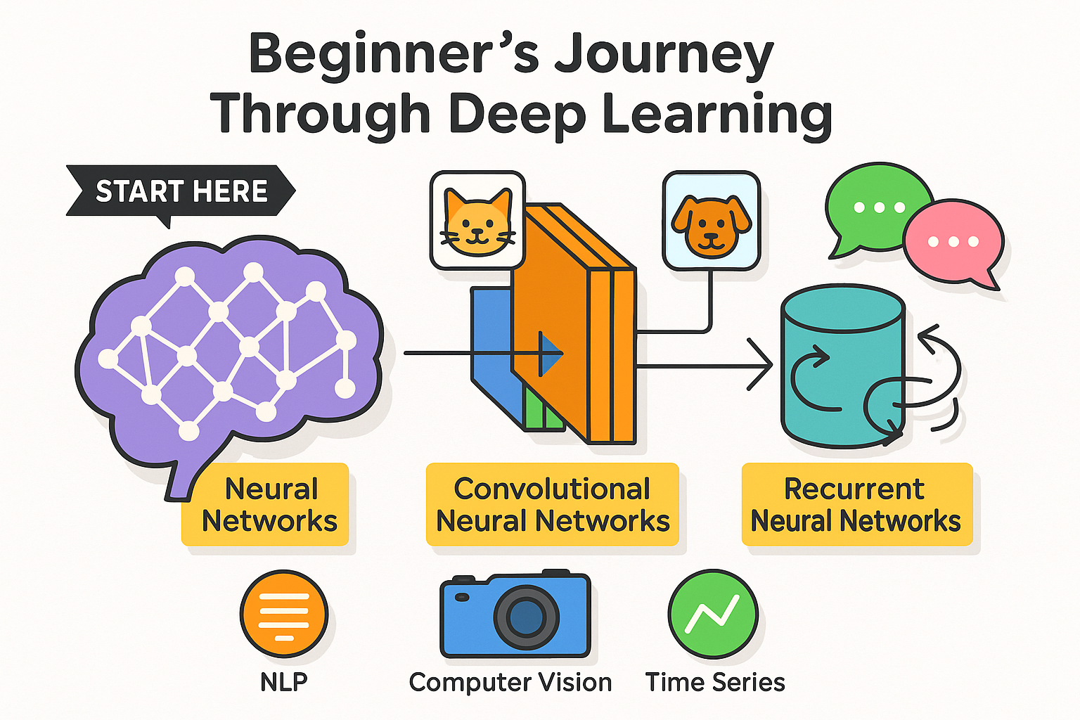
Learning Roadmap
- Start with basic neural networks (perceptrons)
- Move to CNNs for image tasks
- Explore RNNs for sequence data
- Learn NLP fundamentals
- Practice building end-to-end models
- Master evaluation and optimization
- Finally leverage transfer learning
Remember: Deep learning is like learning an instrument – regular practice with small examples leads to mastery over time!
Step-by-Step Explanation of Each Program
(Line-by-line breakdown with detailed explanations for beginners)
1. perceptron.py – Basics of Neural Networks
(A simple perceptron implementing an AND gate logic)
Code Breakdown:
import numpy as np # Import NumPy for numerical operationsnumpyis a library for numerical computing in Python.- We use it for array operations and mathematical functions.
class Perceptron:
    def __init__(self, input_size):
        self.weights = np.random.rand(input_size)  # Initialize random weights
self.bias = np.random.rand() # Initialize random bias__init__: Constructor method that initializes the perceptron.input_size: Number of input features (e.g., 2 for AND gate).self.weights: Random weights (e.g.,[0.3, 0.7]).self.bias: Random bias (e.g.,0.5).
    def predict(self, inputs):
        calculation = np.dot(inputs, self.weights) + self.bias
return 1 if calculation > 0 else 0 # Step activation functionpredict(): Takes input and returns prediction (0 or 1).np.dot(inputs, weights): Computes weighted sum (e.g.,input1 * weight1 + input2 * weight2).+ bias: Adds bias to shift the decision boundary.1 if calculation > 0 else 0: Step function (outputs 1 if sum > 0, else 0).
if __name__ == "__main__":
    perceptron = Perceptron(2)  # Create perceptron with 2 inputs
    perceptron.weights = np.array([1, 1])  # Manually set weights for AND gate
    perceptron.bias = -1.5  # Set bias for AND logic
if __name__ == "__main__":: Ensures code runs only when script is executed directly.perceptron = Perceptron(2): Creates a perceptron with 2 inputs.weights = [1, 1]: Manually set (normally learned via training).bias = -1.5: Threshold for AND gate (ensures0 AND 0 = 0,1 AND 1 = 1).
    test_inputs = [np.array([0, 0]), np.array([0, 1]),
                   np.array([1, 0]), np.array([1, 1])]

    print("AND Gate Results:")
    for x in test_inputs:
print(f"{x} -> {perceptron.predict(x)}")test_inputs: All possible AND gate inputs.for x in test_inputs:: Tests each input combination.perceptron.predict(x): Predicts output (0 or 1).
Expected Output:
[0 0] -> 0
[0 1] -> 0
[1 0] -> 0
[1 1] -> 1
(Matches AND gate logic!)
pip install tensorflow
pip install keras
2. simple_cnn.py – CNN for MNIST Digit Classification
(A basic CNN to recognize handwritten digits from the MNIST dataset)
Code Breakdown:
import tensorflow as tf
from tensorflow.keras import layers, modelstensorflow: Deep learning framework.layers: Contains neural network layers (Conv2D, Dense, etc.).models: Helps in building Sequential models.
def build_cnn():
    model = models.Sequential([
        layers.Conv2D(32, (3, 3), activation='relu', input_shape=(28, 28, 1)),
        layers.MaxPooling2D((2, 2)),
        layers.Flatten(),
        layers.Dense(10, activation='softmax')
])Sequential(): Linear stack of layers.Conv2D(32, (3,3)): 32 filters, each 3×3 (detects edges, textures).MaxPooling2D((2,2)): Downsamples image (reduces computation).Flatten(): Converts 2D features to 1D for Dense layer.Dense(10, activation='softmax'): Output layer (10 digits, probabilities).
    model.compile(optimizer='adam',
                  loss='sparse_categorical_crossentropy',
                  metrics=['accuracy'])
return modelcompile(): Configures model for training.optimizer='adam': Adaptive learning rate optimizer.loss='sparse_categorical_crossentropy': Loss function for classification.metrics=['accuracy']: Tracks accuracy during training.
if __name__ == "__main__":
(train_images, train_labels), (test_images, test_labels) = tf.keras.datasets.mnist.load_data()mnist.load_data(): Loads MNIST dataset (60k train, 10k test images).
    train_images = train_images.reshape((60000, 28, 28, 1)).astype('float32') / 255
    test_images = test_images.reshape((10000, 28, 28, 1)).astype('float32') / 255
reshape((60000, 28, 28, 1)): Reshapes images to (height, width, channels)./ 255: Normalizes pixel values (0-255 → 0-1).
    model = build_cnn()
    model.fit(train_images, train_labels, epochs=2, batch_size=64,
validation_data=(test_images, test_labels))model.fit(): Trains the model.epochs=2: Number of training cycles.batch_size=64: Samples processed before weight update.validation_data: Tests model on unseen data.
3. simple_rnn.py – Time Series Prediction with RNN
(Predicts the next value in a sine wave sequence)
Code Breakdown:
def generate_time_series_data(n_samples=1000, n_steps=20):
    time = np.linspace(0, 100, n_steps * n_samples)
    data = np.sin(time).reshape(n_samples, n_steps, 1)
    X = data[:, :-1]  # All steps except last
    y = data[:, 1:]   # All steps shifted by 1
return X, ynp.linspace(): Generates evenly spaced numbers.np.sin(time): Creates sine wave.reshape(n_samples, n_steps, 1): Formats for RNN (samples, timesteps, features).X = data[:, :-1]: Input sequences (first 19 steps).y = data[:, 1:]: Target sequences (next 19 steps).
def build_rnn():
    model = Sequential([
        SimpleRNN(32, return_sequences=True, input_shape=[None, 1]),
        Dense(1)
    ])
    model.compile(optimizer='adam', loss='mse')
return modelSimpleRNN(32): RNN with 32 memory units.return_sequences=True: Returns output at each timestep (for sequence prediction).Dense(1): Outputs predicted next value.loss='mse': Mean Squared Error (for regression).
    test_sequence = np.sin(np.linspace(0, 2*np.pi, 20)).reshape(1, 20, 1)
    prediction = model.predict(test_sequence)
print("Next value prediction:", prediction[0, -1, 0])test_sequence: New sine wave sequence.prediction: Forecasts next value.
4. nlp_sentiment.py – Sentiment Analysis with NLP
(Classifies text as positive or negative)
Key Steps:
- Tokenization: Converts text to numbers.
   tokenizer = Tokenizer(num_words=100)
   tokenizer.fit_on_texts(texts)
   sequences = tokenizer.texts_to_sequences(texts)
padded_sequences = pad_sequences(sequences, maxlen=5)Tokenizer: Maps words to integers.pad_sequences: Ensures equal length (padding with zeros).
- Embedding Layer:
Embedding(100, 8, input_length=5)- Converts word IDs to dense vectors (learns word meanings).
- Training & Prediction:
   model.fit(padded_sequences, labels, epochs=10)
   test_text = ["This was great"]
   test_seq = tokenizer.texts_to_sequences(test_text)
print(model.predict(test_padded))- Predicts sentiment (0=negative, 1=positive).
5. transfer_learning.py – Using Pre-trained VGG16
(Reuses a trained CNN for custom tasks)
Key Steps:
- Load Pre-trained Model:
base_model = VGG16(weights='imagenet', include_top=False, input_shape=(150, 150, 3))include_top=False: Removes final classification layer.
- Freeze Layers:
   for layer in base_model.layers:
layer.trainable = False- Prevents pre-trained weights from updating.
- Add Custom Layers:
   model = Sequential([
       base_model,
       Flatten(),
       Dense(256, activation='relu'),
       Dense(1, activation='sigmoid')
])- New layers learn task-specific features.
6. model_evaluation.py – Cross-Validation & Metrics
(Evaluates model performance)
Key Steps:
- Cross-Validation:
   scores = cross_val_score(model, X_train, y_train, cv=5)
print(f"Accuracy: {scores.mean():.2f} (+/- {scores.std():.2f})")- Splits data into 5 folds, trains/evaluates on each.
- Classification Report:
print(classification_report(y_test, y_pred))- Shows precision, recall, F1-score.